Divisibles means that the item can be divided to any sizes. A cake is an example.
Goal: Fair and efficient allocation
Model
- $A$: set of $n$ agents
- $M$: set of $m$ divisible goods
- Each agent $i$ has
- Valuation function: $V_i: R_+^m \to R_+$ over bundles of items. (doesn’t have to be linear)
- Concave: Captures decreasing marginal returns (looks like $\sqrt{x}$ curve)
- Allocation $X = (X_1, \ldots, X_n)$ is the allocation of goods to all agents, $X_{ij}$ is the allocation of good $j$ to agent $i$.
Fair (agreeable)
- Envy-free: no agent envies other’s allocation over her own
- For each agent $i$, $V_i(X_i) \geq V_i(X_j), \forall j \in [n]$.
- Proportional: Each agent $i$ gets value at least $V_i(M) / n$ $\equiv$ for each agent $i$, $V_i(X_i) \geq V_i(M)/n$.
Efficient(non-wasteful)
Pareto-optimal: no other allocation is better for all.
- There is no allocation $Y$ such taht $V_i(Y_i)\geq V_i(X_i), \forall i \in [n]$.
Welfare Maximizing: $\max \sum_{i}V_i$ . Doesn’t makes sense sometimes. If a person has very huge values on one thing, should we just give the item to the person?
(Nash) Welfare Maximizing: $ \max \prod_i V_i$. This is the alternative using multipilcations.
Competitive Equilibrium (CE)
Think of Competitive Equilibrium = equilibrium in market
Informally, Demand = Supply $\implies $ CE.
Notation
- Price $p = (p_1, \ldots, p_m)$
- Allocation $X = (X_1, \ldots, X_n)$, $i\in [n], j \in [m], X_{ij}$ is the amount of goods $j$ allocated to agent $i$.
- Valuation functions $V_i(X_i): \mathbb{R}_+^m \to \mathbb{R}_+$is a concave function. (We don’t know if CE exists when $V$ is convex).
We also have a variant of the CE
Competitive Equilibrium with Equal Income(CEEI)
In this model, everyone has the same budget. CEEI has the properties:
An agent can afford anyone else’s bundel, but demands her own $\Leftrightarrow$ CEEI has envy-free property.
By the first welfare theorem $\implies$ Pareto-optimal
Envy-free and “Demand = Supply” $\implies $ proportional
Proof. of the second property.
Say $X = (X_1, \ldots, X_n)$ is the allocation at CEEI. Suppose there is an allocation $Y$ that is Pareto dominating allocation $X$ at CEEI, then $V_i(Y_i) \geq V_i(X_i)$ for all $i \in [n]$, and for some $k$, $V_k(Y_k) > V_k(X_k)$. By CEEI, we also have:
$$ \begin{align*} \sum_{i \in [n]}Y_i \cdot p &\leq \sum_{j\in [m]}p_j && Y_i \leq 1\\ &=\sum_{j \in [m]}p_j \cdot \left( \sum_{i \in [n]}X_{ij} \right) && \text{market clears in CEEI}\\ &= \sum_{i \in [n]} \sum_{j \in [m]} p_j X_{ij} = \sum_{i \in [n]} 1 && \text{budget = 1 for all agent }i\\ &= n \end{align*} $$On the otherhand, since $Y$ PO dominates $X$, we must have for all $i \in [n]$, $V_i(Y_i) \geq V_i(X_i)$. If these $Y_i$’s are affordable (i.e. $Y_i p < 1$), then $Y_i$ would be an affordable bundle that is at least as good as $X_i$, but this contradicts the fact that $X_i$ is the actual demand at CEEI. Therefore, for all $i$, we must have $Y_i \cdot p \geq 1$. Also, $\exists k \in [n]$ such that $V_k(Y_k) > V_k(X_k)$, by the same logic, we must have $Y_k \cdot p > 1$. Summing them up:
$$ \sum_{i \in [n]} Y_i \cdot p > n \cdot 1 $$This brings the contradiction. $\square$
Proof. of the third property
By definition, envy-free means $V_i(X_i) \geq V_i(X_j), \forall j \in [n]$, $\implies$ $n V_i(X_i) \geq \sum_{j \in [n]} V_i(X_j)$.
When demand = supply, the market reaches equilibrium, meaning that the market is clear. Meaning that $\bigcup_{j \in [n]}X_j = M$. Together with concave valuation function $V_i$, we have $\sum_{j \in [n]} V_i(X_j) \geq V_i(M)$. Combining the two inequalities, we get: $V_i(X_i) \geq V_i(M) / n$. $\square$
Now, let’s start by characterizing the CEEI.
Definition(Linear Valuations). $V_i(X_i) = \sum_{j \in M}^{}V_{ij}X_{ij}$, where $V_{ij}$ is agent $i$’s valuation of item $j$, $X_{ij}$ is the corresponding allocation to agent $i$.
The intuition of proceeding to compute CEEI is to spend wisely: spend on goods that gives macimum value-per-dollar (Bang-per-buck), i.e. $V_{ij} / p_j$. We write the inequalities starting from the linear valuation function:
$$ \begin{align} \sum_{j \in M} V_{ij}X_{ij} &= \sum_{j}\frac{V_{ij}}{p_j}(p_j X_{ij}) \\ &\leq \left( \max_{k \in M} \frac{V_{ik}}{p_k}\right) \sum_{j}p_j X_{ij}\\ &\leq \left( \max_{k \in M} \frac{V_{ik}}{p_k} \right) \cdot 1 \end{align} $$With equal income, we simply assume that everyone has the same budget, 1 buck, which is the 1 in step 3. The $\left( \max_{k \in M} \frac{V_{ik}}{p_k} \right)$ is called Maximum Bang-per-Buck (MBB). When do these inequalities become equalities?
Step 2 inequality becomes equality iff the agent buy only MBB goods: $X_{ij} > 0 \implies \frac{V_{ij}}{p_j} = MBB$.
Step 3 inequality becomes equality iff the agent spends all of 1 dollar.
CEEI Characterization
Prices $p = (p_1, \ldots, p_m)$ and allocation $X = (X_1, \ldots, X_n)$ are at equilibrium iff:
- Optimal bundle (OB): for each agent $i$,
- $\sum_{j} p_jX_{ij} = 1$, spend all of 1 dollar
- $X_{ij} > 0 \implies \frac{V_{ij}}{p_j} = \max_{k \in M} \frac{V_{ik}}{p_k} = MBB$.
- Market clear: for each good $j$, $\sum_{i} X_{ij} = 1$.
CEEI Summery
CEEI allocation is:
- Pareto optimal(PO)
- Envy-free
- Proportional
Now, how do we compute CEEI? We focus on a flow based algorithm that can be computed in polynomial time.
Transforming Competitive Equilibrium to Flow problem
Similar to CE, we have the same prices $P = (p_1, \ldots, p_m)$. Then, the “allocation” $F = (f_1, \ldots, f_n)$, where $f_i$ is a vector, and $f_{ij} = x_{ij}p_j$ (money spent by agent $i$ on good $j$).
- Optimal bundle(OB) now becomes:
- $\sum_{j \in M} f_{ij} = \sum_{j \in M} x_{ij} p_{j}= B_i$, where $B_i$ is agent $i$’s budget.
- $f_{ij} > 0 \implies \frac{V_{ij}}{p_j} = \max_{k \in M} \frac{V_{ik}}{p_k} = MBB$
- Market clears now becomes:
- $\sum_{i \in A} f_{ij} = \sum_{i \in A} x_{ij}p_j = p_j\sum_{i \in A} x_{ij}= p_j$, assuming each item has one unit.
Now, consider the following graph with capacity:
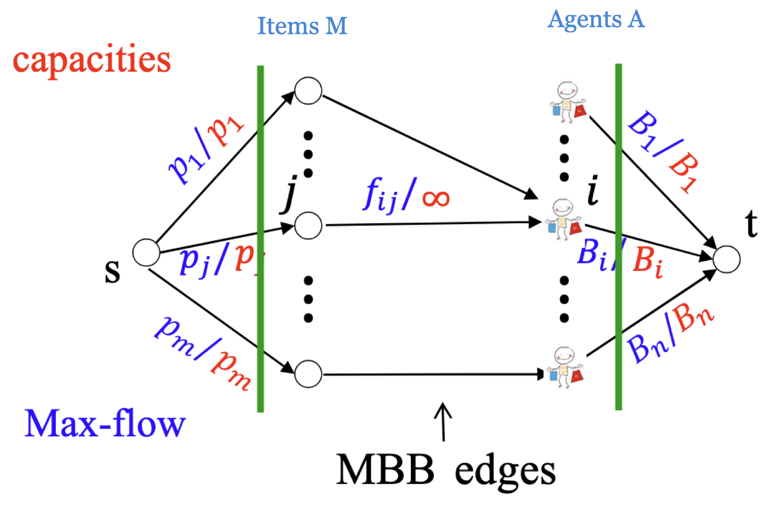
In this graph, an item in $M$ is connected to some agent in $A$ iff the item is an MBB item. In this graph, maxflow = mincut = $\sum_{j \in M} p_j = \sum_{i \in A} B_i$.
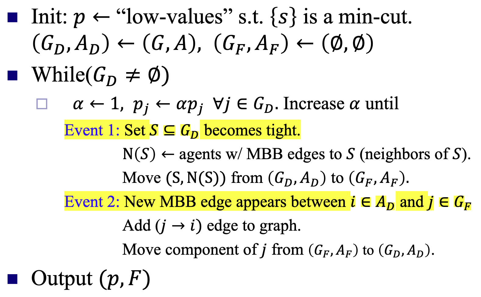
If we know the equilibrium price $P$, we can calculate the “allocation” $F$ easily by allocating the MBB edges. However, we don’t know the price, meaning that we don’t know the MBB edges. The fix is to run [DPSV'08] algorithm.
Idea. We start with low price but keep increasing it. Meanwhile, maintain: (1) flow only on MBB edges, and (2) Min-cut = $\set{s}$ (goods are fully sold). This creates Demand $\geq$ Supply situations.
Check the lecture slide for pictorial description.